Balloon Mapping 1

Introduction

This week the goal was to launch the helium balloon in order to obtain aerial photographs of the campus of the University of Wisconsin-Eau Claire (UWEC). Earlier in the semester we had started to plan out the event by designing the camera carage, weighing out the appropriate payload, and then testing all of the equipment as well. We planned on using our three hour class period to fill the balloon, attach the equipment, and walk around campus to get full coverage. The weather on this particular day was unseasonally cool due to fairly high winds. In the end, the wind played a very big factor in the operation and how well the images turned out. After the camera was recovered, we were to download the imagery and then georeference them to an orthoimage of campus.

Methodology

The first thing that the class did once everyone was together, was to split into different groups; each of which were assigned a different task in the hopes to get the balloon in the air as fast as possible. My group was assigned the task of manning the helium tank down the the first floor of the building and then out to the department's garage outside.

Fig. 1 - Our genius way of transporting the helium tank.

Once we had it in the garage we connected a large piece of clear plastic tubing to the nozzle on the tank and then ran the other end into the bottom of the balloon which was held secure by someone gripping the opening over the tubing while the balloon was filled.

Fig. 2 - Hooking up the plastic tubing to the helium tank.

The filling of the balloon took a good amount of time since we needed to fill it with enough helium to get the balloon's diameter to 5.5 ft. It was important not to overfill the balloon since the balloon expands the higher in the air it goes.

Fig. 3 - Balloon in early stages of being filled.

Fig. 4 - Nearing the 5.5 ft. diameter mark.

Fig. 5 - Hooking up the GPS unit and camera carriage.

Once the balloon was properly filled, we then hooked up a GPS unit to the rig as well as the camera carriage via multiple knots and carabiners. Notice the spool in Fig. 5. This acted as our kite spool, if you will, on which colored marks labeled 50 ft. increments so we knew how high the balloon was.

Fig. 6 - Balloon gaining some altitude as it ascends into the sky.

The camera carriage was a styrofoam worm bucket which was retrofitted to accomodate the digital camera. The camera rig was tied onto the main string a foot or two below the balloon in order to be able to swing freely and obtain images without a string in them.

Fig. 7 - Balloon rig taking some abuse from the wind.

As the balloon got higher in the sky, the wind was blowing it off of its vertical axis. This meant that a large amount of string was being let out and not going straight up. This made it hard to maneuver with the balloon as it was blowing horizontally across campus. The shot in Fig. 7 depicts the balloon around 100 ft. according to the laser range finder we were using. We managed to get around the majority of lower campus and then decided to go across the river via a walkbridge. This is where trouble started. The wind was beating on the balloon so bad it looked like a pancake flopping around. Eventually the string close to the balloon snapped sending the balloon higher into the sky while the camera rig came crashing down into the river. Luckily, it floated close enough to shore where our Professor could snag it with a stick. The good news was that the camera was still working!

Fig. 8 - Pulling the camera rig out of the river.

Fig. 9 - Gathering around the recovered camera rig.

A variety of software was available to us to use to georeference the images: MapKnitter, ArcMap, and Erdas Imagine. An orthoimage of campus was put into the class folder to serve as the reference image. I chose to use MapKnitter since I had never used it before and figured I would try it out since it looked like it was a quick, easy way to georeference.

Results/Discussion

After downloading all of the imagery (over 2,000 images), we soon realized that it would be a difficult task to georeference them and make a quality mosaicked image from them since the shots were very angled from the high winds. The MapKnitter software was very easy to figure out and seemed like a very easy method of georeferencing. The issues I have with the software is that since you're not collecting ground control points (gcp's), I don't think the output is very accurate. Also, I do not know how accurate the reference image is that they provide. I much rather prefer using ArcMap or Erdas for georeferencing since they are desinged to do a more thorough job of georeferencing. The output image I got from MapKnitter isn't terrible considering the quality of the images I had to work with. The bad angles and differing altitudes made it very difficult to get any consistency since the scales varied so much. There is no way that we could have mosaicked the whole campus with these images. Notice how in Fig. 10 some of the sidewalks do not properly line up. With the imagery available it is not the worst thing ever though.

Fig. 10 - Resulting mosaic from MapKnitter.

Conclusion

We learned today that wind is the enemy when trying to conduct balloon mapping. For this reason, the available imagery gathered is not very useful to do any sort of georeferencing or mosaicking. This is rather unfortunate since we put a lot of work into this. However, we were pleased with how long the balloon lasted and that our rig was not a failure. Everything would have worked perfectly had it not been for the wind. Next week we will be launching another balloon with a different rig setup to see if we can get more stability out of it. Hopefully the conditions are more favorable next time so that we can get some high quality imagery to put together.

Final Navigation Exercise

Introduction

This week wraps up our field navigation exercises out at the Priory where we have learned two different types of navigation over the past three weeks: map/compass and GPS. This week we are combining the two methods in order to navigate all three of the courses which means we will be looking for a total of 15 points this week. We were allowed to make new 11" x 17" two sided maps to use for the exercise and then we also brought along our GPS units we used the prior week in order to mark waypoints at each of the flag locations. Another element was added this week to make the navigation a little more interesting. The new element introduced was paintball guns! Each person was issued a Tippman A-5 paintball gun with a hopper full of balls, CO2 tank, and mask. Once again, we retained our groups we have been in during the course of the field navigation exercises. With six teams of three, we would be allowed to choose any route we wanted to find the flag locations, which meant that contact with other teams would be highly likely. The weather for this exercise was excellent with sunny skies and temperatures in the high 30's. The snow levels were around the same as the prior week but this time snowshoes were available for use.

Location

As mentioned above, the final navigation course was held at the Priory, located in Eau Claire, WI, the same location we have been to the last two weeks.

Fig. 1 - The Priory exercise boundary.

The benefit of coming back to this location is that it is pretty familiar by now. We have navigated different parts of the course and know what to expect as far as terrain goes at any point within the exercise area. The area has proved itself to be quite challenging with large elevation changes and dense, wooded areas in parts as well. This familiarity should be beneficial to allow us to navigate all 15 points within the three hour class period. All of the flag locations will hold the same coordinate locations as well. We already have the sheet containing the coordinates in UTM of all 15 flags.

Fig. 2 - Coordinates for all 15 flag locations.

Fig. 3 - Group map for the final navigation exercise.

Methodology

After everyone got to the location around 3:00 PM, we assembled around a small area to get all of the paintball equipment set up and get briefed on what was expected for the field outing. Once all of the equipment was pieced together, it was then passed out to the members of the class. Most people were already familiar with shooting a paintball gun while others took the time to fire off a few practice shots to get the feel for it.


Fig. 4 - Tippman A5 paintball gun used in exercise.

Snowshoes were also made available for this activity and maybe half of the students decided to use them. I chose not to use any snowshoes as I never had before and felt like they might just annoy me more than help me. The teams remained the same as they had for the previous weeks since we were now comfortable working and communicating with the members of our groups.


Fig. 5 - Group member list.

 Each person had a Garmin etrex GPS unit which were to be used for (1) keeping a track log and (2) marking waypoints at each flag. The track log was set up to take a point every 30 seconds. Since all of the teams were gathered in one spot, we were given a three minute grace period to scatter around in the woods before any shooting could begin. We also needed to get a distance away from the Priory building, which serves as a daycare, before we could start shooting as well as not to get the SWAT team called on us.  On our maps, we delineated an area around the building and another facility in the area that we deemed as a "No Shooting" zone.


Fig. 6 - "No Shooting" zones with course points and elevation.



After the three minute window had passed, my team decided to tackle the points from Course 1 and Course 2 first since they were just below the starting location. We managed to get one of the flags (2a) right away with ease and no conflict. On our way to the second flag (3), we encountered some fire from Group 6 as they were on their way to the same point. We sent Kent down the steep ravine to get our card punched as we covered him with supporting fire. Eventually a truce was called upon since we were at a standoff and we were just waisting paintballs and time. Once we had that flag we grabbed flag 3a and then 4 at the northernmost extent of the area. From there we had to walk the steep grade of a hill to get 4a. We decided to leave flag 6b alone for the time since there was another team there who had spotted us so we hiked on over to get 5B. Shortly before we got to 5B, we noticed Group 2 climbing the hill to get it as well. We planned on ambushing them but did not get the chance to before they spotted us. We did not exchange fire but allied with them for awhile. After punching our card at 5B, we decided to grab 5A where we once again ran into Group 6 and a firefight broke out at the edge of the pine tree forest. After exchanging fire from behind skinny pine trees, two of us got hit by their paintballs so we had to sit for 3 minutes before moving on. We were able to then advance to 5A and then over to 4B. After 4B we went to 6A where we met up with Group 2 and Group 6. We exchanged in a short firefight until most of us ran out of paintballs. We then formed a "Mega Group" since we were just about out of time for the exercise. From there we walked to flag 5, dismissing 2B in order to get back in time. On our walk back to the start location, we all got 6b before getting back right around 6 pm. After the exercise, everyone uploaded their track logs into ArcMap in a public folder so everyone could access them. The track logs were then merged together by group members.

Results/Discussion


Fig. 7 - My personal track log.

Animated route from my track log: http://youtu.be/dRO9caw-ovk
 

Fig. 8 - My group's (Group 1) track log and my personal track log.





Fig. 9 - Track logs for all of the groups.



 

In Fig. 7, my track log is shown which gives a better idea of the path I took over the course of the exercise. My track log was turned on at 3:28 pm and turned off when I finished at 5:59 pm. Everyone elses track log times were very similar so I am not going to include those here. Looking at Fig. 8 then with my group's track log and my own laid over the top, it appears that I never really strayed away from my group, which was the case. For most of the exercise, we walked in single file rank the whole time and only spreadout somewhat during the firefights. We took very direct routes to each flag location most of the time. The exceptions would be from 3 to 3a where we took a roundabout way to avoid an ambush and then 4a to 5B because we were trying to ambush Group 2. Other than that, we didn't waste any time getting lost which was good. We should have grabbed flag 2B though since we were super close to it at point 5. Throughout the course exercise, my group only ran into two other groups, Group 2 and Group 6.

 

Fig. 10 - Group 2's track log.

 

Group 2's track log looks pretty confusing in some parts. It appears they managed to get every flag except for 5A. It looks like they may have gotten off track between 3 and 2a and also around 5B; but that is where they ran into us. It looks like they also walked way past point 6 as well, perhaps on their way back to the start location.

 

Fig. 11 - Group 3's track log.

 

Group 3 got to all of the locations except for 2 and 3. It appears their routes were pretty accurate though. I noticed that there is a large break between 6a and 3B. I'm not sure where they started, but it suggests that they started at 3B or 6a perhaps which doesn't make much sense since they are so far away from the start location.

 

Fig. 12 - Group 4's track log.

 

Group 4 made it to all of the points except for 2 and 3 as well. It looks like they strayed off path between 2a and 3a and also around point 5. Perhaps this was due to conflict from other groups.

 

Fig. 13 - Group 5's track log.

 

Group 5 missed four points. These were points 3B, 4B, 5A, and 6. They had pretty good routes too except for around 6a where it looked like they got lost and gave up trying to find 3B or 4B.

 

Fig. 14 - Group 6's track log.

 

Group 6 missed points 2, 6, 5A, and possibly 2B. I know they got 6b because we were in that area at the same time. The reason for the chaos by 3a is because this is where they engaged us in a firefight right away. We also encountered them around 5B in the forest which is why there is some chaos there as well. They must have encountered some conflict between 4B and 6a as well.

 

 

PDOP

 

This concept was covered in the previous blog post but needs to be mentioned in this post as well.  Basically, the PDOP is the accuracy of a 3D position based on the number of satellites and their geometry. A low PDOP indicates a very accurate position. A few of the factors which affect PDOP accuracy are: atmosphere, buildings, and trees. We took a waypoint at each point we went to and then overlaid them on the course points to see how accurately the GPS marked each location. Since this activity took place in an area with lots of trees, the GPS signal was being bounced off the trees and therefore throwing off the correct position of our waypoints in some spots. This is very evident at points 4a and 6b where the waypoint was placed a significant distance from the actual flag location. The GPS is enabled with a feature which helps correct this. The feature is called point averaging and how it works is that the GPS will take multiple points at a location and then average them out to minimize the effect of a high PDOP.

Fig. 15 - Map showing how PDOP involves positional accuracy.

 

 

 

 Conclusion

 

This exercise was a culmination of all the navigation skills we had learned in the past few weeks and gave us a chance to apply them to a course we had gained some familiarity with. In the end, the most effective navigation was by far the GPS. However, it was also very useful to have a paper map along which had an aerial image and contour lines for referencing while in the field. The map showed us the elevation changes we would encounter so that we could plan our navigation for the path of least resistance. Having an aerial image for a base map is also very beneficial to see the type of vegetation in the area and also for identifying landmarks in the event we weren't too sure where we were at. As far as navigation goes though, the map method was antagonizingly slow and inefficient compared to using the GPS. Running around with paintball guns added an extra variable to be aware of. Not only did the masks tend to fog up frequently, we had to be on the lookout for other teams as well which slowed up our navigation a bit. Group 2 probably performed the best based on all of the locations they made it to. No group made it to all of the flags though. It seems like everyone is by now very comfortable navigating with the methods we have learned.

 

 

 

 

 

 

 

 

 

 

 

 

 

 

 

100%

 

 



 

 

 

 

 

 

 

 

 



GPS Navigation Exercise

Introduction

This week's exercise was closely related to the previous week's in that, once again, we were conducting a navigation exercise at the Priory. However, this week we employed a different, more modern technique of navigation. Instead of using a compass and map, all we had with us was a Garmin etrex GPS unit. This type of navigation has several advantages over the map and compass method. First of all, a GPS is way more compact and easy to utilize in the field than is fumbling around with a large map and compass. Secondly, it is way quicker to figure one's location on a GPS as well as finding one's way from point to point because the units are digitally displayed and are calculated in real time. With a map and compass, we had to slowly go through the methodology of figuring out azimuth and then pacing out the distance. This took a long time and got quite frustrating. Thirdly, a user can create a waypoint in the GPS of a particular point and then tell the GPS to find the fastest route to the point. This is a huge advantage over map and compass where the navigator can easily get off path. The only disadadvantage of a GPS is that it could fail in the field if the batteries are bad and then you better hope you packed a map and compass.
The Garmin etrex GPS unit is considered an older unit and can be purchased for relatively cheap. That said, it is still very capable for navigation purposes.

Fig. 1 - GPS unit used in navigation exercise.

Once familiar with the unit settings, the appropriate units should be set before navigating as well as double checking that the appropriate datum is set as well. In this case, the units were set to UTM, which are displayed in meters, which gives the navigator a higher accuracy then does decimal degree units. The datum was left alone at WGS84. In order to see how well we navigated, a track log was set up to display our actual track to each point throughout the course. The track log properties were set to "point", so that every defined time interval, a point was recorded with time and location. This is very useful for post-exercise analysis to be able to map out not only our track, but also to see the times it took to get from point to point. Each member of the group was issued their own GPS unit. It should also be mentioned that in the woods, the density of the forest can affect the positional dilution of precision (PDOP) on a GPS unit. Basically, the PDOP is the accuracy of a 3D position based on the number of satellites and their geometry. A low PDOP indicates a very accurate position. We didn't worry about this variable in this exercise, since we weren't doing any sort of measurements but it can be an important thing to be aware of when using a GPS.

Methodology

Once again, we were to retain our groups we were assigned from last week, but we would be navigating a different course. Each group had to navigate to 6 points, which locations were given to us again. This week Drew Peterson, Kory Dercks, and myself were 15 minutes late getting out to the field because the snow had trapped a certain individuals car in his driveway, hence we had to find another car to get to the field. By the time we got out to the field, the rest of the class had already started navigating. We were told to go to our respective starting points and then catch up to our groups. Drew and I caught up to my group and even though Drew wasn't originally in our group, he decided to stay with us since his group was doing the same course but backwards.

Fig. 2 - Drew Peterson, our adopted group member of the week.

Once all four of us were together, we took some time to debrief each other on how to navigate via GPS. Since we were using a UTM coordinate system, we knew that the coordinate display was showing a northing and an easting. As mentioned before in a previous post on coordinate systems, a UTM zone places the central meridian in the center of the zone and then anything east of the meridian is an easting and anything west of the meridian is a false easting to ensure positive values. Anything north of the meridian is a northing and anything south is a false northing to ensure positive values. For our purposes, all we knew we had to do was watch how the northing and easting values were changing to navigate from point to point. Since we had a sheet with all the points in UTM format, we could determine which way we had to go based on our current location. It's just a matter of knowing that the numbers will increase when moving north or east, or decrease when moving west or south and then figure out the difference from current location and the point location. We found out that it was easiest to match the northing and easting one at a time. What this means is that we would get our easting distance to match and then get the northing to match instead of trying to match both numbers at a time. This was sort of difficult to master at first but then after finding the first point, it became pretty easy.

Fig. 3 - Kent punching his card at the first point location.

 During the navigation exercise, I was playing around with the different functions of the GPS and found out that there was a way easier way to do the navigation. The user can create a waypoint with the point location coordinates and then hit the find button on the GPS interface. This prompts the unit to draw a track on the screen to the point from the current location and tells the user which direction to travel and also how many meters away it is. I don't feel like this is cheating since it is a component of the GPS and is a very effective and efficient way to navigate. We were also very comfortable following easting and northings at by that point anyways.

The navigation conditions were once again rather formiddable. It had snowed pretty heavily the night before which meant that the snow would be deeper this time. We found that in certain spots of the course, snow was knee high. This had a negative impact on the time it took us to navigate. Not only were we traversing through deep snow, but also over very hilly terrain. Most of the course was in the woods but we managed to find a nice road to walk on for different portions between point 4a and 6a. This route also took us along the holding pond of the Priory. This part of the walk smelled awful.

Fig. 4 - Me pointing to the holding pond area.

Fig. 5 - Beatriz taking a break in the snow.

Fig. 6 - Kent finding another flag.

Fig. 7 - Me checking the next point location.

After the field exercise was over with, we took our GPS units to the computer lab where we uploaded our point data into ArcMap. Once the points were in, they were overlaid on top of a high resolution aerial image of the navigation area as well with the points where the flags were located. From here, we were instructed to make 3 maps: our personal track, our group members tracks, and the entire class' tracks.

Fig. 8 - My personal track log.

Fig. 9 - Track logs for our group (1).

Fig. 10 - Track logs for all of the groups.

Discussion

This week, our group successfully navigated through a whole course! We were pretty excited about this since last week's exercise was a navigational fail. This week we felt a lot more comfortable with this style of navigation as most of us had some prior familiarity with GPS navigation. We felt that this style of navigation was way more effective than using compass and map. We were the first group to finish, I believe and within 2 hours on top of that. Just by looking at Fig. 9 above, it is clear that we never really strayed off track at any point of the course. The only hitch we really had was between point 4a and 5a but that was because the dense forest made us change our path vs. being able to navigate in a straight line through the woods. Also, we wanted to be able to follow the road as long as possible since it was easier traveling. Looking at Fig. 10, it looks that every group did a really good job of navigating through their courses as well. Nobody really went too far off track which is really encouraging to see. I think that this shows that the entire class has a good grasp on navigating with a GPS. I think that if we were able to map out our routes from our map and compass navigation exercise, the routes would be all over the place. This proves that a GPS can be a very effective and accurate way to navigate; more so than a map and compass. I wanted to make an animated map of my track log but my GPS unit failed to collect any time data for my points. I am trying to use one of my team members' track log with time data to figure out the animation which would give a really cool graphic of our route.

Navigation with Map and Compass

Introduction

On Monday, March 4th, we conducted our field navigation exercise at The Priory in Eau Claire, WI as mentioned in last week's post. The weather was overcast as we set out to the field around 3:00 PM with a slight drizzle on and off. Upon arrival, we found our respective group members and gathered inside of the building for a quick briefing on the flag locations where we were to navigate to as well as the equipment we would be allowed to use, a compass and our map. The property was large enough to accomodate 3 different courses, each containing 5 flags so that no two teams would be going the same way and thus making each time navigate alone. The courses were overlapped in areas though on purpose to add an extra challenge to make sure that if a flag was spotted from afar, it was not certain that the flag belonged to the course being navigated but could belong to a different course. This was done to ensure that we were following our compasses because a compass never lies, we were told over and over again.

Methodology

Once we were all gathered in the building, we were handed our printed off maps that we created the week before. In addition, we were given the locations of the flags for the course we were to navigate to in the form of UTM coordinates as shown in Fig. 1.


Fig. 1
 

This figure indicates the course number with the respective flag locations as well as the starting point for each course as well. My group was assigned to Course #1. Once we had this information, we started to plot out all the points on the map as well as noting the azimuth for each one based on the previous point. In Fig. 2, everyone is busy plotting their points on their own maps.

Fig 2.

We used the UTM grid on our maps to find the location of each flag and also the starting point. This took some time as we had to double check our map readings and actually ended up plotting 2 points wrong originally so it is definitely crucial to double check or have someone else on your team take a look to get a second set of eyes to ensure accuracy. This could have been very costly and detrimental to our navigation sesssion if we had not caught these mistakes. Figures 3, 4, and 5 depict our team members plotting the points on our maps.

Fig. 3

Fig. 4

Fig. 5

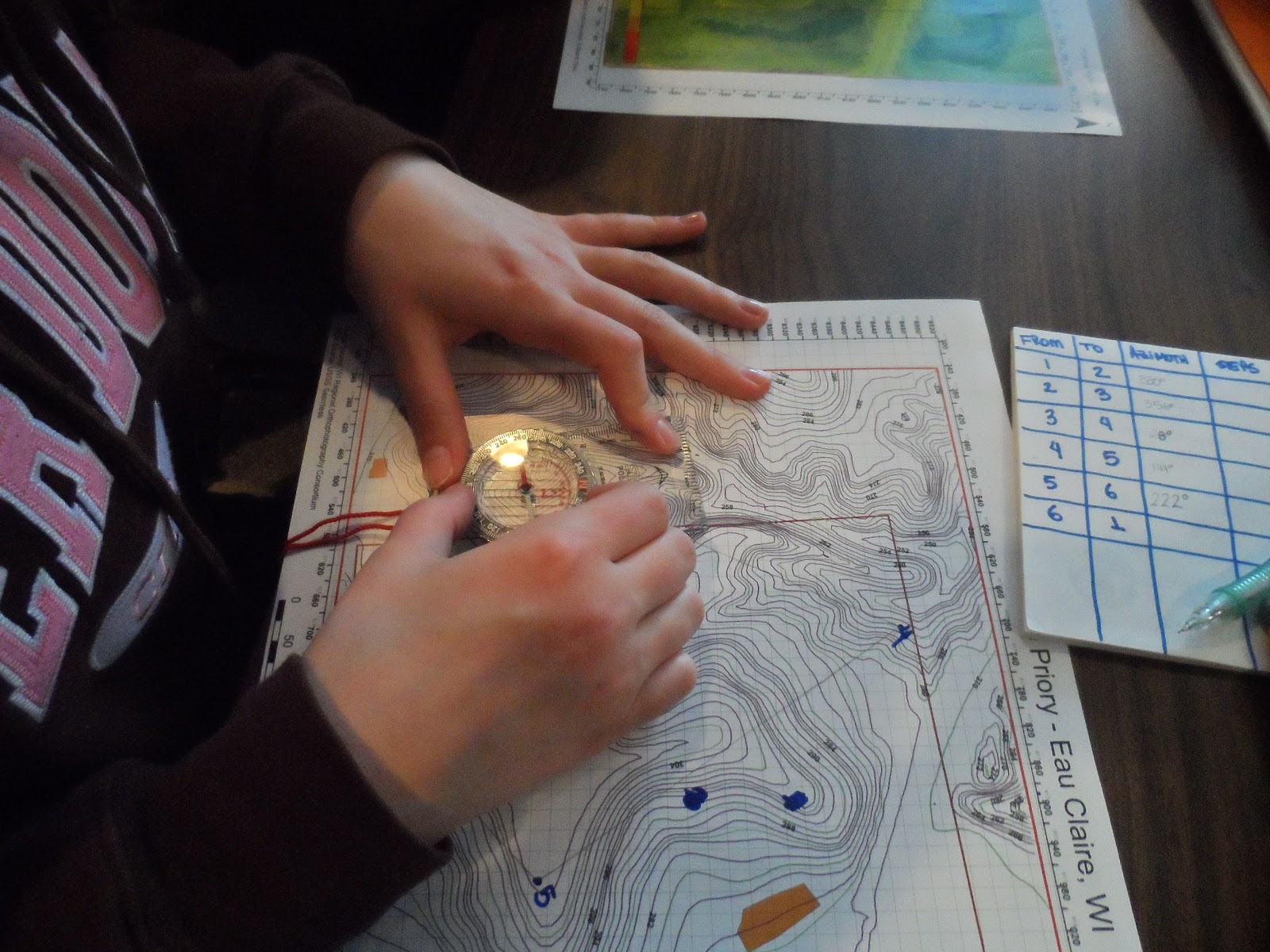
After we finally got all the points in their right locations, we were taught how a compass works and the appropriate way to utilize it. This website does a good job describing how to use a compass along with good graphical instructions as well: http://www.learn-orienteering.org/old/. Each team member was issued a compass so that everyone got practice in understanding and using one. Obviously, it is extremely important to know how a compass works but it is also necessary to be able to get an azimuth from one point to another, using a compass and map. An azimuth is a directional reading based on a circle where 0° or 365° is north and 180° is south, 90° is east, and 270° is west. This sort of preparation is paramount before going out in the field and trying to figure it out there by trial and error. An azimuth was collected from the starting point to the first flag location and then from the first flag location the second location etc...Once out in the field we need this azimuth to determine in which direction to walk. We could estimate the distance to each point by counting the number of grid cells between each point since each grid cell is 20m x 20m. An estimate of distance is very helpful when navigating so one doesn't wander too far. Figures 6, 7, and 8 depict the process of plotting points on a map and then calculating an azimuth based off of a straight line between points. Also, in Fig. 7 and 8, the elevation range is shown which clued us in to the range of elevation we would experience in locating the flags.

Fig. 6

Fig. 7

Fig. 8

Once we had all of the prep work done for the activity, which took around an hour, we headed outside to the starting point for our course. From there it was just us with a map and compass and the wilderness which is shown in Fig. 9.

Fig. 9

 The snow was still pretty deep throughout the woods and it became readily apparant that I should have worn boots instead of shoes. Anyways, this is basically what we had to navigate through, along with challenging elevation changes. Once at the starting point, we assigned one person to man the map and stay at the starting point, another person to walk a distance in the azimuth direction to a landmark (usually a tree), and then the third person to count paces from the point to where the second person was standing. We thought this would be the most effective way to stay on the right track because it is very easy to get off the correct path when there are trees in your way. Also, we applied the pace count we took the week before to get an estimate how many meters we had walked so that we had a general idea of how close we should be to the flag. Once again, this was not super accurate because we could not walk in a straight line as we had done in the control experiment but was still very helpful we found out. Navigation to the first point went fairly smoothly even though we had to descend a pretty steep incline to reach it. Figure 10 shows a bit of our navigation to the first point. Here I am counting paces between where my partner Beatriz is standing, pointing out the azimuth and where my other partner Kent is, a landmark along the azimuth.


Fig. 10

Fig. 11 depicting more pace counting between Beatriz and Kent

Fig. 12 - Getting deeper into the thicket, suppressing quick navigation.

We were not able to move very quickly through the forest due to the abundance of trees and the deep snow. However, we managed to stay relatively close to the azimuth and only ended up 11 paces to the west of where the flag was. Needless to say, we were pretty pumped and group morale was at an all time high.

Fig. 13 - The flag from where we first spotted it.

Fig. 14 - Kent (left) and I celebrating our find! Great success!

Fig. 15 - False Flag (tree marker)

Morale was soon to take a hit while navigating to the second flag however. To get to the second flag, we had to descend further down into the valley, and a little further than we had to travel from starting point to flag #1. We applied the same strategy as we had done for the first point as it worked out very well for us. At this point, it should be mentioned that my feet were completely soaked and cold, but I continued on. We walked the distance that we felt we needed to go, but saw no flag anywhere so we walked further until we got to a deep ravine. Still, nothing. Beatriz and myself decided to stay at the point where we felt the azimuth and distance were correct and sent Kent out to explore the perimeter. After a time, Kent came back stating that he did not see anything. We then split up and walked all around the area near the ravine since that is where it looked like it should be on our contour map. We ended up wandering around for a good half hour before we decided that maybe we should go back to flag #1 and start over in case we miscalculated the azimuth. At this point, Martin the field supervisor, came by and told us we should look at the bottom of the ravine. We went to the same spot that we originally thought it would be and looked down to the bottom of a very steep ravine, and sure enough, the flag was pretty much at the bottom of the ravine. Here we learned a valuable lesson: always trust your compass. All we failed to do was look all the way down.

Fig. 19 - Point 3 (flag #2) shown atop elevation contours.

At this point, it was getting dark so Martin instructed us to follow him around to the rest of the points so that we could complete the course before it got dark. We did this and then got back to base camp around 6 pm. It turned out that our group and another were the only ones not to finish our course. This was very disappointing to hear. We had the rest of the week to reflect on our outing and figure out what went wrong and why.

Discussion

We all learned a great deal about navigation with a compass and map from the field outing. We started off strong with our navigation exercise, but failed to complete the course after just finding one flag which was very frustrating. One of the issues that was brought up between our group was that we had not really observed the elevation changes too well on our maps which caught us off-gaurd once in the field. Our maps should have shown more detail with the elevation so that it would have been a bit more obvious that flag #2 was far down a ravine. In Fig. 19, the contour lines are 2m intervals, but we should have gone finer detail with the contours. We were following the correct line, but just failed to realize that the flag was all the way down the ravine, not near the edge where it looks like it is on our maps. I blame myself for not using finer contour lines as well as not breaking up the DEM elevations into more classes which led to over generalization of the elevations. Another thing, as mentioned above, is to never second guess your compass. We doubted our compass because we did not see the flag at first, which led us to wander around aimlessly in the woods with the slim hopes of getting lucky and blindly running across the flag. Next time I need to be more prepared for the physical elements of the field by wearing boots and not shoes. Being unprepared for such elements can greatly hinder effective navigation and could also prove to be fatal if alone in the cold. Our method of navigation was very effective though, with each person assigned a different task to keep everyone on track. It is a bit burdensome trying to manage a compass on top of a paper map in the field, but it can be extremely effective though if that is one's only option. Given another shot at the course, we are very confident that we could find all of the flags. I was pretty excited to be able to navigate with a compass though, since I had never done this before. It is a very valuable skill to learn and actually quite simple once one is able to apply it to a field setting. This week, we will be out in the same area doing navigation with a GPS, using lat./long. coordinates instead of UTM



.














 



 

 

Field Navigation Map

Introduction
This week's assignment is preparing the class for a field navigation outing at the University's new daycare center, a few miles south of campus, denoted by the place marker here in Fig. 1.

Fig. 1

The total land area that this exercise will take place on is approximately 112 acres in size and consists of hilly and woody terrain. A high resolution aerial image is shown in Fig. 2 with a red boundary box denoting the area in which various points will be placed for the class to navigate to.


Fig. 2

For this exercise, we won't have any fancy navigational instruments such as a GPS, but rather we will be relying on the old school technique of map and compass to find various points scattered around the plot of land. Often times, a GPS might lose it's signal if one is in dense vegetation or maybe the batteries will run out when in the field. Then what? It is vital to be able to navigate without reliance on technology. Knowing how to use a map and compass is a fail proof way to ensure that if in a sticky situation when technology fails, one can find their way to any point on the map. Teams will be split up into teams of three, so once in the field, one person will be walking, the second person navigationg the walker, and the third person manning the compass and map. Each member of the group is responsible for creating a map (front and back) on an 11" x 17" piece of paper. Out of the three, we will agree on which one we will use for the field navigation exercise.

Methodology
The first thing we did in preparation for the navigation exercise was to go outside and conduct a pace count. Essentially, a pace count is a way to count how many steps one takes in a 100 meter stretch. This will become extremely helpful since we won't have a GPS unit to establish an exact distance for us. It should be noted that we conducted the pace count on a sidewalk to get a true 100 meter distance. However, it is also apparent that once in the woods, we won't be able to walk in a straight line, therefore we will have to add a few paces to our own pace counts to adjust to the situation we will face in the woods. Everyone did the pace count at least twice so that we could average our paces if they were off each time we did it. My personal pace count was 67 paces per 100 meters. Also, the reason that we did this exercise in meters is because our maps will utilize a UTM coordinate system which also measures distances in meters.

That being said, let's talk coordinate systems for a bit! Coordinate systems are the single most important part of making a map. One must know which coordinate system is best suited for their area of interest or else the map could become useless or even work against you. Most people are familiar with the standard latidude/longitude coordinate systems, but rarely should this coordinate system be used outside of making a small geographic scale or global map. This is because latitude and longitude cannot be used to measure precise distances which are needed in a navigation situation. Thus, for surveying or navigation uses, a coordinate system suited for a large geographic scale are necessary. The most popular and useful are UTM and State Plane coordinate systems which allow meter precision. A UTM coordinate system breaks the world into longitudinal based strips or zones in order to minimize distortion. More information on UTM coordinate systems can be found here: http://egsc.usgs.gov/isb/pubs/factsheets/fs07701.html.
A State Plane System is a coordinate system developed specifically for each state. The only problem with this is that this system is still considered to broad for an area like the one we will be doing our field activity on. A State Plane system is best suited for an area covering most of a state or an area falling between two UTM zones within a state. We decided that utilizing a UTM coordinate system would suit us best for our exercise. The exercise area falls into UTM zone 15 and we will use the NAD83 datum for reference.

The next step was to compile all of the data we will be using for making our map into a file geodatabase in ArcMap so that we could run the Arctools and spatial analysis tools on the files. Our geodatabse consists of: shapefiles for navigation and point boundaries, orthoimagery of the area of interest, surveyed 2 ft. contour lines, and also a DEM. After getting all of the data into the geodatabase, it is necessary to get all of the data into the same projection so that further analysis can be done accurately. Once again, we wanted to get all of the data into the UTM 15N projection. This is where we hit a bit of a speed bump with the surveyed contour data. This data was in a CAD format and lacked any spatial projection reference as shown in Fig. 3.



Fig. 3

 

 

 

We were unable to succesfully define a projection for this dataset, so we had to follow a specific order of adding layers. First, we had to add our projected orthoimage which then set the data frame projection to UTM 15N so that if any more layers are added, they are automatically projected on the fly to UTM 15N. This does not mean that the projection is defined or changed for the CAD file however, it just allows the dataset to overlay where it should if it had a defined projection of UTM 15N. This is a really nice feature of ArcMap. It is suggested though that even though a dataset lacking projection properties that is projected on the fly, one cannot do any further analysis until the projections are the same in the properties window. To avoid this headache, our group decided that we did not really need to use 2 ft. contour intervals, so we scrapped that dataset. What we did instead was use the DEM and run a spatial analyst tool to make contours set at whatever interval we wanted. We chose to use 2 meter intervals because this size interval will still give us elevation detail but not clutter the map up so much. Fig. 4 shows how cluttered the 2 ft. contour intervals would have made the map. 

Fig. 4

Since the elevation range in this area is from 245m - 312m, it is really not necessary for our purposes to have this detailed of contour lines because it just makes the map more confusing and busy which will distract from effective navigation. All of the various datasets were clipped to fit the Navigation Boundary box so that there was no extra, unneeded data showing.

The map that I made, which was chosen for the group map, is detailed in the following paragraph and images.
For the one side of the map (Fig. 5), I wanted just a basic, clean map showing the contour lines along with the prominent man-made features of the landscape: the Children's Center, two houses in the SW, and a holding pond to the NE highlighted in orange. The purple contour lines are the 2m contours and the green contours are 5m contour lines. I was also able to label each contour line for quick reference. The Children's Center building sits atop the highest elevation point. The inside red square box indicates the point boundary and the outer, thicker red box indicates the navigation boundary. We included a 20m x 20m grid over the top of the map elements so measuring distances will be very easy. Other map elements include: North arrow for reference, scale in meters, and also projection information. 



Fig. 5

On the other side (Fig. 6), I chose to include the orthoimage which will be very helpful for visual reference of the landscape and also a color coded DEM to show the altering elevations of the landscape.

Fig. 6

I left the grid on top as well and then labeled both ends of the elevation legend bar which is incremented into 10m segments. The red areas are the highest elevation and the dark green are the lowest elevations. The goal was to keep the maps simple yet effective and I think that these maps meet the criteria and will be very useful in the field for navigation.

Discussion
The key concepts from this exercise include datasets, map projections, and map elements. All three are extremely important as they each contribute vital information to the map itself and also to the user. One has to decide on what datasets are most important to the map reader and then how to manipulate the datasets to show what you want as well as to create an aesthetically pleasing and useful map. Once again, projections make or break a map. Firstly, make sure to pick an appropriate coordinate system and then make sure all of the datasets are defined to the same projection to provide an accurate range of data. Map elements such as a north arrow, scale, and some sort of legend are also vital elements of map. Without these elements the map becomes very ambigous and useless. These maps will be put to the true test this coming week as we will actually be out in the field implementing them. I just hope these maps work well or my group may start a mutiny against me!