Using ArcPad to Collect Field Data

Introduction

The final exercise of the semester involves collecting data using a mobile device. In this particular instance, a Trimble Juno GPS will be used in conjunction with ArcPad to collect field data at the Priory. We have spent a good amount of time this semester out at the Priory, which is a plot of land recently purchased by the University of Wisconsin - Eau Claire, which is now a daycare center. Other than the daycare center, the rest of the property is occupied by forest with ever changing topography. There are some trails evident but have not been properly kept up and the trails are poorly marked in spots.

Fig. 1 - Trimble Juno GPS used to collect the field data.

The goal of this assignment was to collect certain types of features at the Priory so that the data could be compiled into useful maps. Being able to understand and employ ArcPad in the field is a crucial asset as this has become a very popular way for companies to collect data in the field. After the data collection is complete, the data will be uploaded into ArcGIS where feature classes will be created and then overlaid on top of a high resolution aerial image.


Study Area

Fig. 2 - The Priory is approximately a 4 mile drive from the University of Wisconsin - Eau Claire campus.



Fig. 3 - Aerial photo of the Priory - Eau Claire, WI.

The total land area that this exercise will take place on is approximately 112 acres in size and consists of hilly and woody terrain.


Methodology

In order to efficiently complete the field work in a 3 hour time period, the class split up into 6 groups.

Fig. 4 - Groups and their respective members. 

 Some of the features that were assigned to different groups were: Trails (type, condition), Trail Markers (color, shape), Benches (condition, azimuth), Erosion Points, Fallen Trees (lying over trails), Animal Tracks, Birdhouses, and Garbage (piles of garbage or abandoned equipment). After each group knew what they would be mapping, we needed to setup a geodatabase in ArcMap. The geodatabase was named appropriately and assigned the coordinate system NAD_1983_HARN_Wisconsin_TM. Once the preliminary steps of creating the geodatabase was complete, we added two point feature classes to it: Benches and Markers. Since each feature class had different criteria possibilities, it was necessary to create fields and domains for each feature. For Benches, this meant including an Azimuth field ranging from 0-365, and a Condition field with options Good, Fair, and Poor to describe the bench's condition. For Markers, a field was created for Shape (no domain was set for this), Medium (wood, metal, or other), and Color (no domain was set for this either). The fields where no domain was set is because we were not sure how many different colors were used for trail markers or how many different shapes there were. Because of this, we did not want to limit our options by creating a domain. However, we could still be able to manually type in the text values on ArcPad in the field. The benefit of using domains is that defined values can be used to mitigate manual entry error.

After we had defined all of the conditions, it was time to export the geodatabase onto a Juno GPS unit. This can be done through the ArcPad Data Manager Toolbar.

Fig. 5 - The ArcPad Data Manager toolbar in ArcMap 10.1.

By clicking on the Get Data button, circled in red, the wizard takes you through the steps for getting the data ready for ArcPad. This involves defining the folder path to where the data will be stored. An ArcPad map project will be made with a .apm file extension. After this, the data will be deployed to the appropriate folder. The next step is to connect the Juno to the computer via USB cable. The deployment folder can then be pasted onto the SD card inside the Juno. It is best to check the Juno to make sure the process was completed properly before heading out to the field. So no we have the geodatabase containing the feature classes on the Juno as well as an aerial basemap which will run in the background. The basemap is optional as it is useful but can bog down the system.

Once we arrived at the Priory, all we needed to do was wait for a GPS signal lock and then we took to the woods to start collecting data. After a half hour of data collection, it was evident that with all of the trail markers on the trees, it would take more than our allotted class period to collect all of the data. We split the group up so that I would collect all of the triangle shaped trail markers, Kent would collect the circle shaped markers, and Beatriz would collect the benches. This proved to be a way more efficient way of collecting the data and we had it all collected within 2 hours. Once, the data collection was complete, we headed back to the computer lab to upload the data into ArcMap. A tool called Bearing Distance to Line was run on the Benches feature class in order to show the azimuth of the view from each bench. We did not collect data on the view distance from each bench so a standard 25m distance was given to each bench. The important thing here is that we can see which way the bench is positioned.

The data was saved on the Juno as an .ssf file which is not directly supported in ArcMap. In order to convert this to a shapefile, we had to employ the ArcPad Data Manager once again. This time, we clicked on the Add Data icon and uploaded the .ssf file. From there, it recognized our Benches and Markers features. We clicked both of them and then clicked the "Check in" button which updated our reference geodatabase with the new attribute data for our features.

Fig. 6 - Updating the geodatabase with feature point data collected with ArcPad.

Results/Discussion

Fig. 7 - Trail markers and benches at the Priory.

Fig. 8 - Zoomed in look at the trail markers and benches.

The first time employing an ArcPad project into the field was very successful. There were a few groups who lost their data in transition from the field to computer. We were lucky enough to retain all of our data. We were able to gather all of the data we originally set out to in the allotted time. We ended up with 51 trianle markers, 51 circle markers, and 6 benches. It looks like the benches are spread around the trails in a very even manner. It is a bit confusing determining what the triangle and circle markers differentiate. We only saw one sign indicating a trail name. Also, it was quite common to see a triangle marker on one side of the tree and a circle marker on the other side. Perhaps the different shapes indicate the direction of travel on the trail. Now that they are mapped, the coordinator at the Priory can clear up this confusion. We also entered attribute data for the condition of the markers as well indicating if they are clearly visible, need paint, or if they are on a fallen tree of which a few were.

Conclusion

This exercise was beneficial in two ways. First of all, we got invaluable experience with another component of ESRI software in ArcPad. This sort of skill is highly marketable as this is a very popular method in data collection. Secondly, the types of data and the detail it was collected in, both spatially and attribute, will help the coordinator at the Priory with improving the trail conditions. Maps containing multiple datasets can be made to allow visitors to navigate with ease and allow them to have an enjoyable time exploring the woods at the Priory.

High Altitude Balloon Launch (HABL)

Introduction

The objective this week was to launch our HABL rig into the upper atmosphere with a camera recording the journey. Typically, balloons such as these, reach altitudes of 60,000 to 120,000 ft which would be located in the stratosphere. The stratosphere is the second major layer of the Earth's atmosphere, sitting atop of the troposphere. The stratosphere is characterized by cool temperatures near the bottom and warmer temperatures higher up which is the direct opposite of the troposphere where the warmer air is located near the surface and cools as altitude increases. This is because the Earth's atmosphere is warmed from below from trapped radiation from the sun. This temperature inversion becomes important in regards to launching a balloon that high because the equipment (camera, GPS) will be exposed to very cold temperatures and thus need to be protected with insulation. Since helium is lighter than air, the balloon will rapidly ascend, expanding as it rises. Eventually the expansion of the gas inside the balloon will be so great that it will cause the balloon to burst. The ascent of the balloon can be controlled by how much helium is inside the balloon. Since the weather has been very inclement this spring, it was a gamble on when we could launch our rig. We finally got a nice day on Friday 4/26 with temperatures around 70°F and a slight wind which prompted us to launch the balloon.

Methodology

We had been preparing for this day on and off the past few months. Earlier on in the semester, we researched balloon types, weighed out a payload, and made a few rig designs so that we would be prepared for launch day. Around 8:30 a.m. on 4/26, some of the class arrived at school to fill the balloon with helium and to secure the parachute and camera rig to the balloon. The camera was placed in a square styrofoam container with a lens hole cut in the bottom in order to allow a clear area of view for recording.

Fig. 1 - The camera carriage being constructed.

 Hand warmers were shaken to activate the heat which would keep the camera from freezing up at high altitudes. A flip camera was used as the recording device which supports up to an hour of video recording. The rig is suspended from rope on each side, approximately 3 ft. length, and then the pieces are tied together at the top so that the carriage can swing freely in flight. Pieces of packaging tape were used to fasten the lid on the bottom so that the camera would not fall out during the course of the flight. The camera carriage was fastened to the balloon via carabiners. The balloon was larger than the one used for the aerial mapping exercises we performed over the last few weeks. It was necessary to get a larger balloon for this exercise as it would be required to obtain higher altitudes. The diameter of the balloon after filling it with helium exceeded 8 feet. We did not want to fill it to the max as the balloon would need room to expand as it rises. Once the balloon was filled to the desired level, we fastened the neck of the balloon with a few zip ties and then folded it over on itself and duct taped it liberally. A small GPS tracking device was also attached to the rig so that we would be able to locate the signal of where the rig lands. The camera carriage and parachute were then fastened and then we walked the HABL rig out to the center of campus to launch it.

Fig. 2 - Transporting the HABL rig to the launch pad.

Results/Discussion

With a wind around 12-15 mph from the west, the balloon took off rather quickly from the launch pad in an easterly direction. The balloon managed to gain altitude rather quickly as it was blown away. After a few minutes, we lost sight of it and headed back inside to await a signal from the tracking device. Over an hour passed before we finally got a signal from the tracking device telling us that the rig had landed in a field near Marshfield, WI which is a little over an hour away from where we launched it. There were some strong high level winds which carried the HABL a distance of 78 miles!  The complete video is posted below. The camera took an hour's worth of video and shut off shortly after the descent.

http://desi.uwec.edu/Geography/Hupyjp/Weather_Balloon_1024.asx (Here is a quick link until I can get the video embedded into the blog)

Fig. 3 - A still frame of a shot above the campus of UWEC.

Fig. 4 - The balloon has ascended quite high at this point as the field of view has increased dramatically.

Fig. 5 - The balloon close to its highest altitude taking an image off nadir allowing us to view the horizon.

Fig. 6 - This still frame is my favorite image. How awesome is it that the balloon reached this height and captured this awesome image! At this point the air is very thin and the balloon probably popped shortly after. 

Fig. 7 - The balloon got caught in the canopy of a tree 50 ft. off of the ground on its way back down to Earth. 

Fig. 8 - Professor Hupy recovers the camera carriage after free climbing the tree and sawing off the branch the rig was hung up on. 

Fig. 9 - The balloon started to travel in a northwest direction from the launch location as it passed over the U.S. 53 bypass.

Fig. 10 - The HABL rig is passing by Lake Eau Claire here, about 20 miles from the launch location and has since switched to a southeasterly direction of movement.

Fig. 11 - The HABL covered approximately 78 miles in its journey before landing in the country near Marshfield, WI.

Conclusion

This exercise was probably my favorite one this semester as it was awe-inspiring to see the results from the HABL flip camera. I have never even considered an opportunity where I could be a part of a project sending an object that high into the air and being able to recover video from it. Looking at the still frames from 100,000 ft. is just mind boggling. I wish that the camera rig had been more stable throughout the flight as it can be very nauseating to watch the video with everything spinning so fast. A popular idea on fixing camera stability on a balloon rig is that of a gyro-stabilized contraption so that the camera remains in a fixed position as the unit rotates with the balloon. This would be immensely helpful for the next launch as the video quality would be much improved and more still frames could be extracted. The other limitation of this launch was the camera being used. The Flip Cam could only record up to an hour of video which ended up cutting out much of the descent. A GoPro camera would be ideal for this sort of application as it is more rugged and can record for a much longer time as well as providing stunning video quality. These changes will require more money but would be well worth it as the end product would be that much better. A proposal has also been stated that for the next launch, there should be a camera taking video in the near infrared (NIR) to get satellite quality imagery. Also, a thermometer, barometer, and anemometer should be sent up with next time as well to collect temperature, pressure, and wind speeds at different altitudes to better understand the upper atmosphere. There are a lot of really cool and practical applications that this sort of project can be used for. The event was profiled by a local paper as well which can be read here: http://www.uwec.edu/News/releases/13/05/0507HABL.htm.

Balloon Mapping II

Introduction

This week we conducted another balloon launch in the hopes to get better aerial photographs. The weather was a lot more cooperative this time around as there was virtually no wind. The skies were a bit overcast but we were hoping that this would not affect the color quality of the images. We decided to make a few changes to the camera carriage this time as to provide more stability. The location we were mapping again was the campus of the University of Wisconsin-Eau Claire (UWEC).

Fig. 1 - The UWEC campus we covered with the balloon and camera.

A walk to cover an area of this size took around 2 hours. Factored into this was dodging tree branches, power lines, and crossing streets.

Methodology

Once again, the class split into small groups to tackle different tasks in order to expedite the preparation process. This included transporting the helium tank outside to the garage, hooking up the fittings, filling the balloon, and then fastening the camera rig to the balloon. We got rid of the old camera carriage (styrofoam bucket) in exchange for a newly engineered carriage which featured a harness and arrow for stability. The arrow would act as a wind vane, steering the camera while keeping it steady while the camera shoots pictures every 3 seconds. Unfortunately we did not get any photos of the new camera carriage. Once the balloon was filled to the appropriate size, it was quickly launched into the air. We had a team of 3 manning the balloon spool to keep track of how much line was out and also to better control it as it was walked around campus. The group walked the balloon over different sections of campus in order to get full coverage.

Fig. 2 - Launching the balloon rig into the air.

A 32MB SD card was put into the camera to ensure the memory would not fill up at some point during our exercise. After we were satisfied with the area we covered with the balloon, we took it down and retrieved the camera and subsequently downloaded the imagery onto a lab computer. In all, we had 5,000 images to sort through! The next task was to georeference enough images to cover the entire campus area. We decided it would be more practical to split campus up into different sections and assign groups of 3 to each section. Each group would mosaic their images together and upload them to a class geodatabase where all the mosaics would be mosaicked to a new raster covering the entire study area.

Results/Discussion

The imagery obtained from this exercise was far better than the imagery we got from the previous week. This was due to calmer conditions and a more stable camera carriage. Once the balloon reached peak altitude of 400 ft. (approximately), it held very steady and was basically completely vertical. The only issue we had to deal with in the images was the balloon string. This happened because the camera was nestled right next to the string the whole time and so the string was constantly in the camera viewer.

Fig. 3 - A shot from around 400 ft. in the air.

Fig. 4 - Collecting imagery of the new academic center under construction.

Fig. 5- A shot near the river.

Some of the imagery looks a bit washed out but the overall quality is definitely usable. The biggest thing is that the camera is taking images almost off of nadir, a bit oblique in some.

Georeferencing

Since these images do not contain any spatial reference, they need to be assigned the correct geographical location so that they can be mosaicked together and displayed properly. In order to do this, one needs to find an image that is spatially correct. These images are commonly referred to as orthoimages. An orthoimage (Fig. 1) was provided to the class to be used as the reference image for the georeferencing process. There were two options available to us to conduct the georeferencing: ArcMap and Erdas Imagine. I chose to use ArcMap to conduct the georeferencing even though I do have experience georeferencing in Erdas as well. In ArcMap, you need to open up the Georeferencing toolbar to get started.

Fig. 6 - The georeferencing toolbar in ArcMap

From there load in the orthoimage first so that spatial data is defined in the Layer data. The next step is to drop the image (JPEG) into the viewer as well. The JPEG will not show up on top of the orthoimage because it still lacks spatial data. We are now ready to collect ground control points (gcp's). GCP's are used to match features from the unreferenced image to the orthoimage and then the image will be assigned the correct spatial data after enough gcp's are collected. It is important to collect a gcp from the unreferenced image first and then place one in the same spot on the orthoimage. The best points to collect gcp's are at the vertices of features such as sidewalks or corners of parking lots. It is not a good idea to use corners of buildings in this case since the angle on the images are not the same as the angle on the orthoimage. Doing this will screw up the georeferencing. The user has a choice between using a first order, second order, or third order polynomial transformation. A first order polynomial transformation is best fitted for images that do not exhibit a great deal of distortion. A minimum of 3 gcp's must be collected for this transformation. A second order polynomial transformation is best suited for images that have a noticeable amount of distortion. This transformation will warp the edges of the image more in order to get the proper plane. A third order polynomial transformation is for severely distorted images and is not used very often. I started out using first order polynomial and collected around 20 gcp's on my first image. I got a fairly low root mean square (RMS) error. The RMS error let's the user know how well the gcp's match on the two images. Generally, an RMS error below 0.5 is desirable.

Fig. 7 - Table containing the RMS error total for all 22 gcp's.

I was able to switch to second order polynomial through the properties tab and this greatly improved the alignment of the image. It turned out that the JPEG images were warped enough to need the second order transformation. The area of upper campus that my group was assigned to wasn't too bad to correct as there were enough features to collect gcp's on over the whole scene of the JPEG image. If you don't spread out your gcp's, there will be distortion in certain areas. I was quite pleased how well the geometric correction went on the first image.

Fig. 8 - This image shows the JPEG being georeferenced to the orthoimage.

I ran the same process for 5 more JPEGs that encompassed my area. Once they all were georeferenced to my liking, I exported them as a .tif, and now they contained the correct spatial data. After this was done, the next step was to run a mosaic to stitch the images together.

Mosaic

A mosaic is a way to combine a number of separate rasters (TIF, JPEG,etc...) into a new seamless raster. There are two options for mosaicking in the ArcMap toolbox: Mosaic and Mosaic to New Raster. Running the Mosaic tool is not suggested as it overwrites one of the input rasters. After you run the mosaic, the original reference image is lost and has now become the completed mosaic. This is not good, especially if the tool does not run correctly at first. The best option is to use Mosaic to New Raster since this will create a new raster from the input files and not overwrite any of them so you retain the originals if something goes wrong. All of the images to be mosaicked should be loaded into the data frame so that they can be stacked or tiled correctly so that the best image is on top. The tool will recognize the top image properties and use them on the overlap areas so that the images are seamlessly stitched together.

Fig. 9 - The Mosaic to New Raster tool dialog box.

The tool will take some time to run the more images there are so be patient. After the mosaic process is complete, look over the output to make sure it is to your liking or else you will have to re run the mosaic with a different stack order. Once all the group members have their mosaics completed, they will then be mosaicked together to make one large, high quality image of campus!

Fig. 10 - Mosaic overlaid on top of orthoimage.
 

There is still a bit of work to do to find an image that can overlay this mosaic which would hide the balloon string.

Conclusion

Overall, this week's activity went much smoother than the previous week's. This time it was nice to get consistent angles on our images so that they weren't too distorted. Using professional software such as ArcMap or Erdas allows for way more accurate georeferencing. It was good to practice these types of skills on a challenging project like this. It will be interesting to see how everyone else did on their mosaics and if they are consistent with everyone else's or else we may run into some problems with the mosaics lining up correctly. This is always a concern when there is a number of different people working on different areas of the image because not everyone has the same level of experience and so consistency may be thrown off. It is nice to have the work split up though because it would take one person a very long time to be able to georeference and mosaic enough images to cover the whole study area by themselves.

Balloon Mapping 1

Introduction

This week the goal was to launch the helium balloon in order to obtain aerial photographs of the campus of the University of Wisconsin-Eau Claire (UWEC). Earlier in the semester we had started to plan out the event by designing the camera carage, weighing out the appropriate payload, and then testing all of the equipment as well. We planned on using our three hour class period to fill the balloon, attach the equipment, and walk around campus to get full coverage. The weather on this particular day was unseasonally cool due to fairly high winds. In the end, the wind played a very big factor in the operation and how well the images turned out. After the camera was recovered, we were to download the imagery and then georeference them to an orthoimage of campus.

Methodology

The first thing that the class did once everyone was together, was to split into different groups; each of which were assigned a different task in the hopes to get the balloon in the air as fast as possible. My group was assigned the task of manning the helium tank down the the first floor of the building and then out to the department's garage outside.

Fig. 1 - Our genius way of transporting the helium tank.

Once we had it in the garage we connected a large piece of clear plastic tubing to the nozzle on the tank and then ran the other end into the bottom of the balloon which was held secure by someone gripping the opening over the tubing while the balloon was filled.

Fig. 2 - Hooking up the plastic tubing to the helium tank.

The filling of the balloon took a good amount of time since we needed to fill it with enough helium to get the balloon's diameter to 5.5 ft. It was important not to overfill the balloon since the balloon expands the higher in the air it goes.

Fig. 3 - Balloon in early stages of being filled.

Fig. 4 - Nearing the 5.5 ft. diameter mark.

Fig. 5 - Hooking up the GPS unit and camera carriage.

Once the balloon was properly filled, we then hooked up a GPS unit to the rig as well as the camera carriage via multiple knots and carabiners. Notice the spool in Fig. 5. This acted as our kite spool, if you will, on which colored marks labeled 50 ft. increments so we knew how high the balloon was.

Fig. 6 - Balloon gaining some altitude as it ascends into the sky.

The camera carriage was a styrofoam worm bucket which was retrofitted to accomodate the digital camera. The camera rig was tied onto the main string a foot or two below the balloon in order to be able to swing freely and obtain images without a string in them.

Fig. 7 - Balloon rig taking some abuse from the wind.

As the balloon got higher in the sky, the wind was blowing it off of its vertical axis. This meant that a large amount of string was being let out and not going straight up. This made it hard to maneuver with the balloon as it was blowing horizontally across campus. The shot in Fig. 7 depicts the balloon around 100 ft. according to the laser range finder we were using. We managed to get around the majority of lower campus and then decided to go across the river via a walkbridge. This is where trouble started. The wind was beating on the balloon so bad it looked like a pancake flopping around. Eventually the string close to the balloon snapped sending the balloon higher into the sky while the camera rig came crashing down into the river. Luckily, it floated close enough to shore where our Professor could snag it with a stick. The good news was that the camera was still working!

Fig. 8 - Pulling the camera rig out of the river.

Fig. 9 - Gathering around the recovered camera rig.

A variety of software was available to us to use to georeference the images: MapKnitter, ArcMap, and Erdas Imagine. An orthoimage of campus was put into the class folder to serve as the reference image. I chose to use MapKnitter since I had never used it before and figured I would try it out since it looked like it was a quick, easy way to georeference.

Results/Discussion

After downloading all of the imagery (over 2,000 images), we soon realized that it would be a difficult task to georeference them and make a quality mosaicked image from them since the shots were very angled from the high winds. The MapKnitter software was very easy to figure out and seemed like a very easy method of georeferencing. The issues I have with the software is that since you're not collecting ground control points (gcp's), I don't think the output is very accurate. Also, I do not know how accurate the reference image is that they provide. I much rather prefer using ArcMap or Erdas for georeferencing since they are desinged to do a more thorough job of georeferencing. The output image I got from MapKnitter isn't terrible considering the quality of the images I had to work with. The bad angles and differing altitudes made it very difficult to get any consistency since the scales varied so much. There is no way that we could have mosaicked the whole campus with these images. Notice how in Fig. 10 some of the sidewalks do not properly line up. With the imagery available it is not the worst thing ever though.

Fig. 10 - Resulting mosaic from MapKnitter.

Conclusion

We learned today that wind is the enemy when trying to conduct balloon mapping. For this reason, the available imagery gathered is not very useful to do any sort of georeferencing or mosaicking. This is rather unfortunate since we put a lot of work into this. However, we were pleased with how long the balloon lasted and that our rig was not a failure. Everything would have worked perfectly had it not been for the wind. Next week we will be launching another balloon with a different rig setup to see if we can get more stability out of it. Hopefully the conditions are more favorable next time so that we can get some high quality imagery to put together.

Final Navigation Exercise

Introduction

This week wraps up our field navigation exercises out at the Priory where we have learned two different types of navigation over the past three weeks: map/compass and GPS. This week we are combining the two methods in order to navigate all three of the courses which means we will be looking for a total of 15 points this week. We were allowed to make new 11" x 17" two sided maps to use for the exercise and then we also brought along our GPS units we used the prior week in order to mark waypoints at each of the flag locations. Another element was added this week to make the navigation a little more interesting. The new element introduced was paintball guns! Each person was issued a Tippman A-5 paintball gun with a hopper full of balls, CO2 tank, and mask. Once again, we retained our groups we have been in during the course of the field navigation exercises. With six teams of three, we would be allowed to choose any route we wanted to find the flag locations, which meant that contact with other teams would be highly likely. The weather for this exercise was excellent with sunny skies and temperatures in the high 30's. The snow levels were around the same as the prior week but this time snowshoes were available for use.

Location

As mentioned above, the final navigation course was held at the Priory, located in Eau Claire, WI, the same location we have been to the last two weeks.

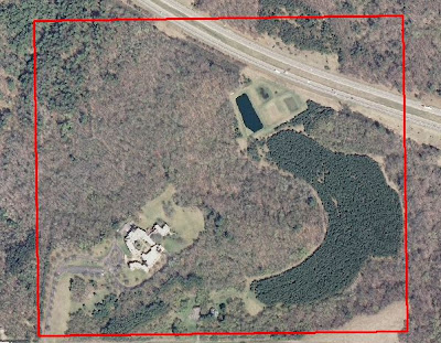
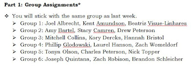
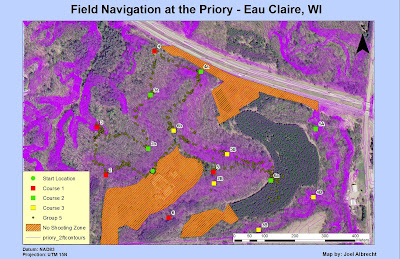
Fig. 1 - The Priory exercise boundary.

The benefit of coming back to this location is that it is pretty familiar by now. We have navigated different parts of the course and know what to expect as far as terrain goes at any point within the exercise area. The area has proved itself to be quite challenging with large elevation changes and dense, wooded areas in parts as well. This familiarity should be beneficial to allow us to navigate all 15 points within the three hour class period. All of the flag locations will hold the same coordinate locations as well. We already have the sheet containing the coordinates in UTM of all 15 flags.

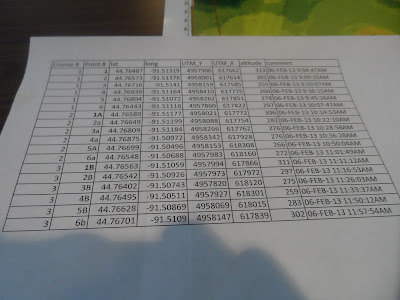
Fig. 2 - Coordinates for all 15 flag locations.

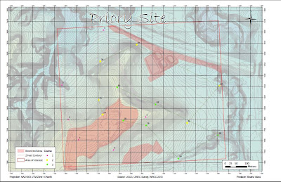
Fig. 3 - Group map for the final navigation exercise.

Methodology

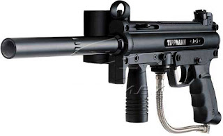
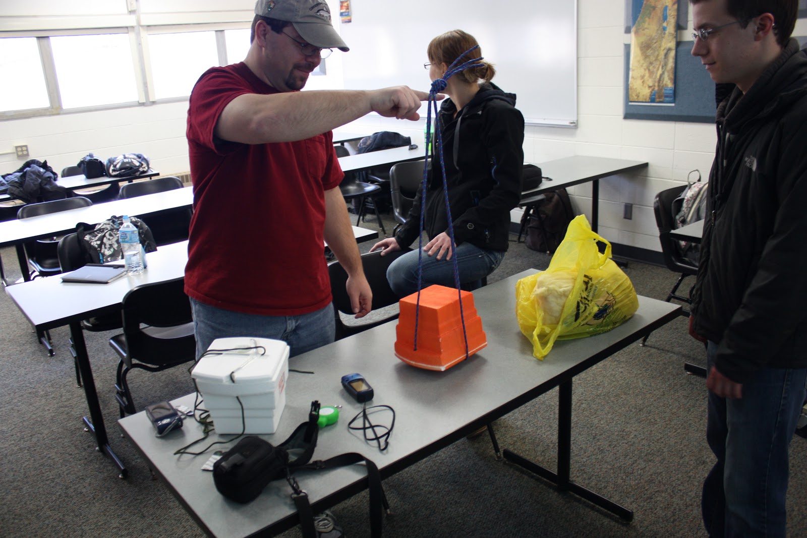
After everyone got to the location around 3:00 PM, we assembled around a small area to get all of the paintball equipment set up and get briefed on what was expected for the field outing. Once all of the equipment was pieced together, it was then passed out to the members of the class. Most people were already familiar with shooting a paintball gun while others took the time to fire off a few practice shots to get the feel for it.


Fig. 4 - Tippman A5 paintball gun used in exercise.

Snowshoes were also made available for this activity and maybe half of the students decided to use them. I chose not to use any snowshoes as I never had before and felt like they might just annoy me more than help me. The teams remained the same as they had for the previous weeks since we were now comfortable working and communicating with the members of our groups.


Fig. 5 - Group member list.

 Each person had a Garmin etrex GPS unit which were to be used for (1) keeping a track log and (2) marking waypoints at each flag. The track log was set up to take a point every 30 seconds. Since all of the teams were gathered in one spot, we were given a three minute grace period to scatter around in the woods before any shooting could begin. We also needed to get a distance away from the Priory building, which serves as a daycare, before we could start shooting as well as not to get the SWAT team called on us.  On our maps, we delineated an area around the building and another facility in the area that we deemed as a "No Shooting" zone.


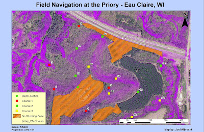
Fig. 6 - "No Shooting" zones with course points and elevation.



After the three minute window had passed, my team decided to tackle the points from Course 1 and Course 2 first since they were just below the starting location. We managed to get one of the flags (2a) right away with ease and no conflict. On our way to the second flag (3), we encountered some fire from Group 6 as they were on their way to the same point. We sent Kent down the steep ravine to get our card punched as we covered him with supporting fire. Eventually a truce was called upon since we were at a standoff and we were just waisting paintballs and time. Once we had that flag we grabbed flag 3a and then 4 at the northernmost extent of the area. From there we had to walk the steep grade of a hill to get 4a. We decided to leave flag 6b alone for the time since there was another team there who had spotted us so we hiked on over to get 5B. Shortly before we got to 5B, we noticed Group 2 climbing the hill to get it as well. We planned on ambushing them but did not get the chance to before they spotted us. We did not exchange fire but allied with them for awhile. After punching our card at 5B, we decided to grab 5A where we once again ran into Group 6 and a firefight broke out at the edge of the pine tree forest. After exchanging fire from behind skinny pine trees, two of us got hit by their paintballs so we had to sit for 3 minutes before moving on. We were able to then advance to 5A and then over to 4B. After 4B we went to 6A where we met up with Group 2 and Group 6. We exchanged in a short firefight until most of us ran out of paintballs. We then formed a "Mega Group" since we were just about out of time for the exercise. From there we walked to flag 5, dismissing 2B in order to get back in time. On our walk back to the start location, we all got 6b before getting back right around 6 pm. After the exercise, everyone uploaded their track logs into ArcMap in a public folder so everyone could access them. The track logs were then merged together by group members.

Results/Discussion


Fig. 7 - My personal track log.

Animated route from my track log: http://youtu.be/dRO9caw-ovk
 

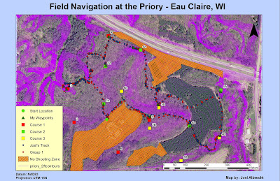
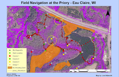
Fig. 8 - My group's (Group 1) track log and my personal track log.





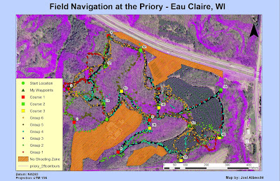
Fig. 9 - Track logs for all of the groups.



 

In Fig. 7, my track log is shown which gives a better idea of the path I took over the course of the exercise. My track log was turned on at 3:28 pm and turned off when I finished at 5:59 pm. Everyone elses track log times were very similar so I am not going to include those here. Looking at Fig. 8 then with my group's track log and my own laid over the top, it appears that I never really strayed away from my group, which was the case. For most of the exercise, we walked in single file rank the whole time and only spreadout somewhat during the firefights. We took very direct routes to each flag location most of the time. The exceptions would be from 3 to 3a where we took a roundabout way to avoid an ambush and then 4a to 5B because we were trying to ambush Group 2. Other than that, we didn't waste any time getting lost which was good. We should have grabbed flag 2B though since we were super close to it at point 5. Throughout the course exercise, my group only ran into two other groups, Group 2 and Group 6.

 

Fig. 10 - Group 2's track log.

 

Group 2's track log looks pretty confusing in some parts. It appears they managed to get every flag except for 5A. It looks like they may have gotten off track between 3 and 2a and also around 5B; but that is where they ran into us. It looks like they also walked way past point 6 as well, perhaps on their way back to the start location.

 

Fig. 11 - Group 3's track log.

 

Group 3 got to all of the locations except for 2 and 3. It appears their routes were pretty accurate though. I noticed that there is a large break between 6a and 3B. I'm not sure where they started, but it suggests that they started at 3B or 6a perhaps which doesn't make much sense since they are so far away from the start location.

 

Fig. 12 - Group 4's track log.

 

Group 4 made it to all of the points except for 2 and 3 as well. It looks like they strayed off path between 2a and 3a and also around point 5. Perhaps this was due to conflict from other groups.

 

Fig. 13 - Group 5's track log.

 

Group 5 missed four points. These were points 3B, 4B, 5A, and 6. They had pretty good routes too except for around 6a where it looked like they got lost and gave up trying to find 3B or 4B.

 

Fig. 14 - Group 6's track log.

 

Group 6 missed points 2, 6, 5A, and possibly 2B. I know they got 6b because we were in that area at the same time. The reason for the chaos by 3a is because this is where they engaged us in a firefight right away. We also encountered them around 5B in the forest which is why there is some chaos there as well. They must have encountered some conflict between 4B and 6a as well.

 

 

PDOP

 

This concept was covered in the previous blog post but needs to be mentioned in this post as well.  Basically, the PDOP is the accuracy of a 3D position based on the number of satellites and their geometry. A low PDOP indicates a very accurate position. A few of the factors which affect PDOP accuracy are: atmosphere, buildings, and trees. We took a waypoint at each point we went to and then overlaid them on the course points to see how accurately the GPS marked each location. Since this activity took place in an area with lots of trees, the GPS signal was being bounced off the trees and therefore throwing off the correct position of our waypoints in some spots. This is very evident at points 4a and 6b where the waypoint was placed a significant distance from the actual flag location. The GPS is enabled with a feature which helps correct this. The feature is called point averaging and how it works is that the GPS will take multiple points at a location and then average them out to minimize the effect of a high PDOP.

Fig. 15 - Map showing how PDOP involves positional accuracy.

 

 

 

 Conclusion

 

This exercise was a culmination of all the navigation skills we had learned in the past few weeks and gave us a chance to apply them to a course we had gained some familiarity with. In the end, the most effective navigation was by far the GPS. However, it was also very useful to have a paper map along which had an aerial image and contour lines for referencing while in the field. The map showed us the elevation changes we would encounter so that we could plan our navigation for the path of least resistance. Having an aerial image for a base map is also very beneficial to see the type of vegetation in the area and also for identifying landmarks in the event we weren't too sure where we were at. As far as navigation goes though, the map method was antagonizingly slow and inefficient compared to using the GPS. Running around with paintball guns added an extra variable to be aware of. Not only did the masks tend to fog up frequently, we had to be on the lookout for other teams as well which slowed up our navigation a bit. Group 2 probably performed the best based on all of the locations they made it to. No group made it to all of the flags though. It seems like everyone is by now very comfortable navigating with the methods we have learned.

 

 

 

 

 

 

 

 

 

 

 

 

 

 

 

100%